

For two decades, negative stock–bond correlation made asset allocation look cleaner than it was. Equities carried growth; Treasuries rallied when growth broke and policy eased. That relationship powered 60/40 portfolios, risk parity, rebalancing and leverage.
Since 2022, the mechanism has run in reverse. Inflation raised discount rates and financing costs at the same time, pushing stocks and bonds down together. The portfolio problem is no longer how many asset classes we own. It is how many independent shocks the portfolio can survive.
1. Negative correlation was a regime, not a law
The long history is clear: the deeply negative stock–bond correlation of 2000–2020 was unusual. Correlation was positive through much of the twentieth century, especially when inflation and the term premium dominated growth risk.
When growth breaks, policy rates fall and Treasuries can hedge equity losses. When inflation surprises higher, both the discount rate and the cost of capital rise. Stocks and bonds then share the same enemy.
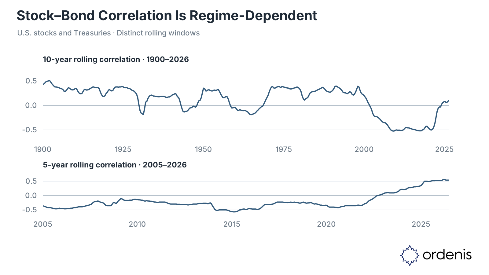
The negative episodes also had different causes. The 1930s were deflationary. During the 1940s, rate caps partly detached bond prices from the growth outlook. The post-2000 regime lasted much longer because inflation expectations were anchored and crises were interpreted mainly as growth or financial shocks. The hedge worked because the macro regime supported it.
2. What 60/40 actually owns
A 60/40 portfolio is less diversified than its labels suggest. The bond sleeve reduces volatility, but equity risk still drives most of the result.
In the reconstructed long sample, annualized volatility was roughly 18.35% for stocks, 5.51% for Treasuries and 11.13% for a monthly rebalanced 60/40 portfolio. The same calculation from 2022 produced 16.73%, 6.68% and 10.95%. Bonds still dampened the ride; they did not create an independent return engine.
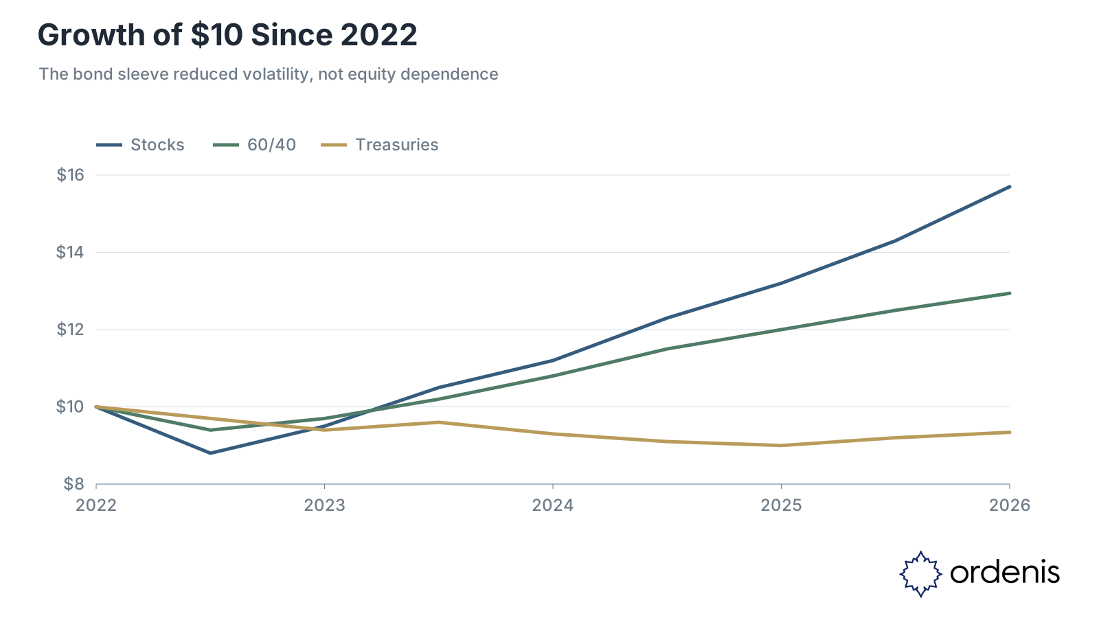
The distinction is between capital weight and risk weight. Forty per cent of the dollars can sit in bonds while equities still explain most of the variance. That is why the rolling correlation of 60/40 with stocks remains close to one.
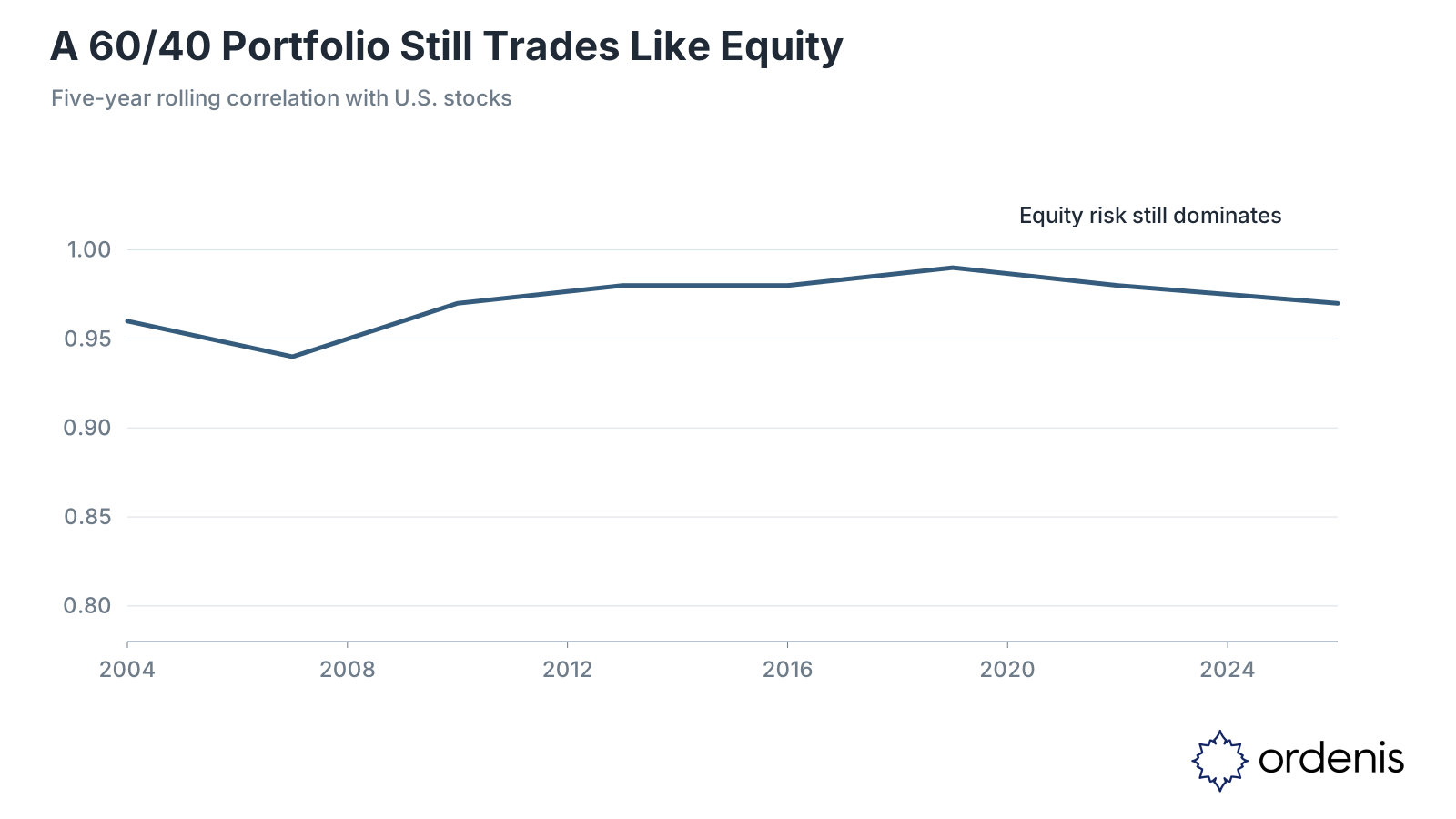
Bonds remain useful. They hedge growth recessions, deflation and duration-matched liabilities. What they do not provide is unconditional insurance against every drawdown.
3. Diversify shocks, not names
Once correlation rises, asking for a “bond replacement” misses the point. The right question is which shock the portfolio does not currently hedge.
Treasuries and cash still work when growth collapses. They work less reliably when the shock is inflation, supply scarcity or a rising term premium. The missing exposure must then come from another return source.
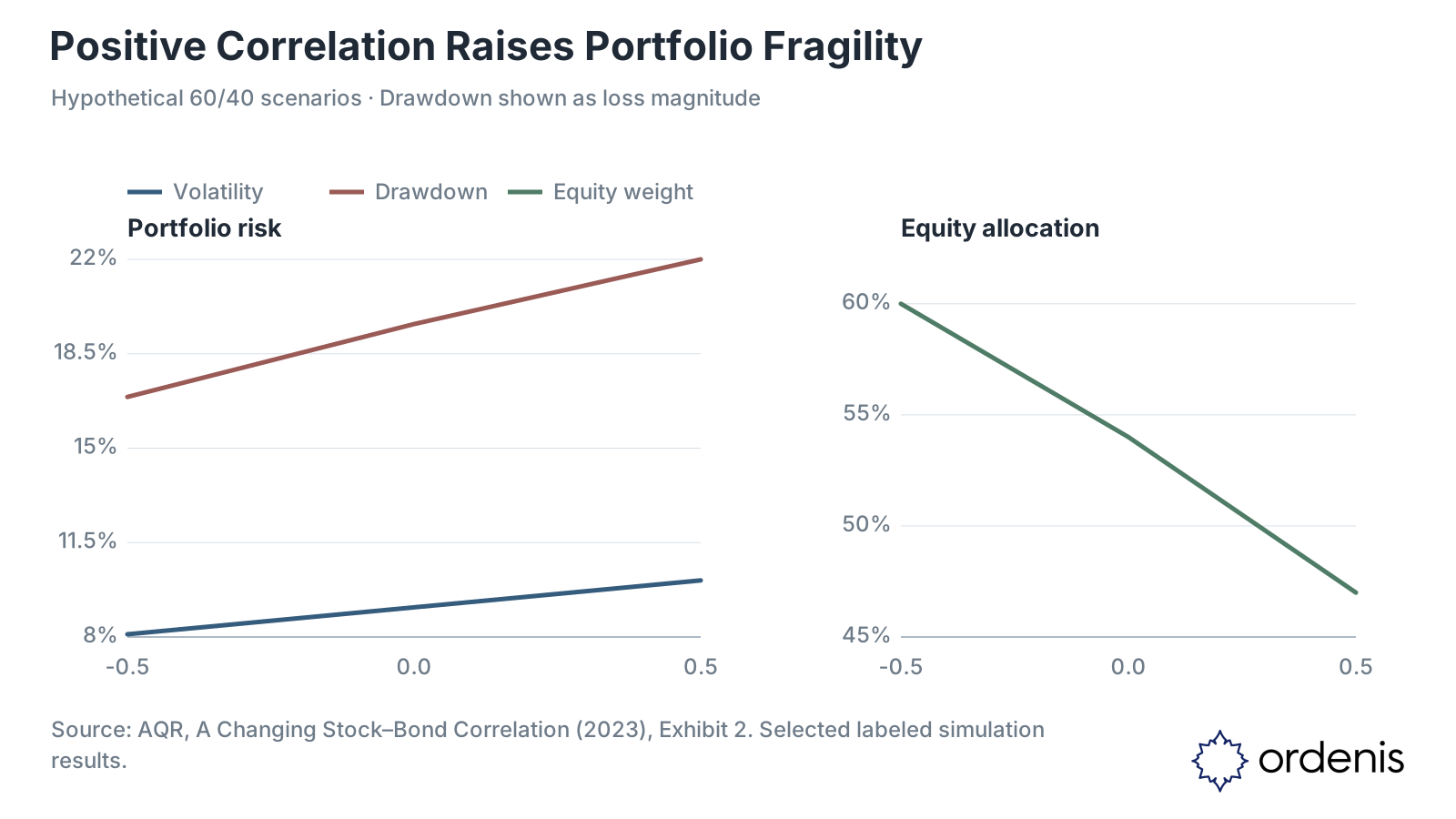
In AQR's hypothetical scenario analysis, moving stock–bond correlation from −0.5 to +0.5 raises portfolio volatility from 8.1% to 10.1% and the reported largest-drawdown magnitude from 16.9% to 22.0%. Holding the original risk budget forces the equity weight down from 60% to roughly 47%. Without a new diversifier, stability is purchased by giving up return.
TIPS, commodities and gold are not interchangeable. TIPS defend real purchasing power but can fall when real yields rise. Commodities respond to spot scarcity and inventories, with meaningful carry. Gold responds to real rates, the dollar and monetary credibility. The edge comes from combining distinct failure modes, not from declaring one asset the new bond.
4. Build around risk sources
A more robust framework separates growth, inflation, real rates, credit and liquidity, then adds strategies whose P&L is not tied to a rising market. Trend, relative value, market-neutral exposures and convex protection can each solve a different part of the problem.
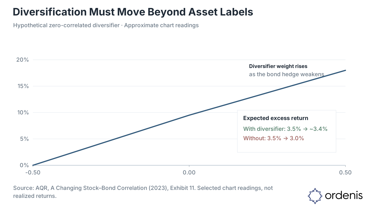
The AQR framework assumes annual volatility of 15% for stocks, 4% for bonds and 10% for the alternative, with a 0.3 Sharpe ratio for each. The alternative is uncorrelated with both stocks and bonds. These are model assumptions, not forecasts for a specific strategy. Study and methodology.
Optimization should test four distinct losses: growth recession, inflation, a rate shock and a funding squeeze. Liquidity, margin, borrowing cost, negative carry and concentration by risk source belong inside the constraints. A portfolio with a lower full-sample Sharpe can be better built if it avoids failing for the same reason everywhere.
The final test is behavioral, not cosmetic. If a supposed hedge develops a rising equity beta, falls in the target stress or owes its low volatility to stale marks, it is a return asset and should be sized as one.
The objective is not to make every period profitable. It is to stop every position from losing under the same macro shock.